Top Cut
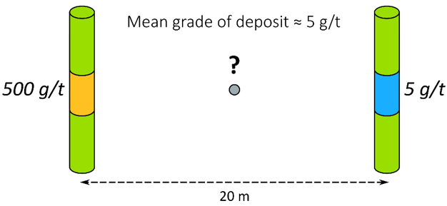
Consider the drillholes shown below. The interval on the left intersected a coarse nugget that assayed 100 times higher than the mean grade of the deposit. However, nuggets are very rare, and you would not expect to the same high grade if you were to twin the hole.
Top-cutting high grades to minimise high-grade bias
If you were to naïvely estimate the grade between the two samples, you might assume that they contribute equally to the result. But this simple average would produce an unrealistic value of 250 g/t, spreading the tiny high-grade nugget across 20 m. Cutting the 500 g/t assay to a more representative value minimises that effect.
By capping higher grades to the top cut value, you use a more conservative grade in the interpolation, minimising the risk of overestimating the grade. You should not use a top cut with non-linear methods like multiple indicator kriging (MIK).
Handling Valid High Grades
The top cut value can be hard to determine when the data includes extreme but otherwise valid values, and because of this uncertainty it is important to determine the cut value using as many methods as possible for each element in each domain. Although the results of the different methods are unlikely to agree, an informal weight-of-evidence assessment should reveal a range of preferred values. You may also choose to omit the top cut altogether if your data does not include any outliers.
You use the Top Cut chart to assess potential top cut values by combining up to nine of the following methods on a single chart. You then select the top cut candidates in each chart and compare them with the others:
- Histogram: If abnormally high grades appear as a distinct population in the histogram, use statistical decomposition to determine the boundary value, which then becomes the cut value.
- Cumulative Frequency curve or Probability Plot: Look for break-up near the right-hand end of the graph. The grade at which the graph breaks up is the cut value.
- Mean vs. Top Cut: Inspect the plot for a change in slope, which may indicate a change in sensitivity to the cut value.
- Relative Nugget vs. Top Cut: Assesses short-scale continuity as defined by the relative nugget. Look for the minimum value within a zone of coherent points, which indicates the best grade continuity.
- Quantile Analysis: Assesses the individual quartiles in the dataset, working through a series of rules that indicate if a top cut is warranted. See: Quantile Analysis
To preserve the original sample values for verification and auditing, always apply the top cut to a new field via the File Editor Calculations (Expression) button, or the Calculate (Expression) tool on the File tab, in the Edit Data group.
![]()
Use the expression =CUTHIGHS([GradeField], Cut) to apply the top cut, replacing GradeField with your grade fieldname and Cut with your top cut value.