Cross Validation
![]()
Cross validation is a way of testing the validity of the model prior to using it for Kriging or IDW Estimation. The operation is also known as “jack-knifing” although statisticians sometimes use that term for a different procedure.
The difference between the estimated value and the actual value is used to calculate the standard error of the estimate and the error statistic. The function calculates the ratio of the actual error (actual value – estimated value) to the standard deviation to obtain the standard error. If the basic assumptions have been satisfied and you have chosen the correct semi variogram model, the average error statistic should be zero and the standard deviation of the error statistic, one.
When you run Cross Validation, it calculates the standard error for each point and displays it in Vizex. The purpose of the Cross Validation display is to highlight data values that differ markedly from their modelled values.
Sample Location, True vs. Estimate, Standard Error, and Standard Error vs. Estimate charts can also be generated to assess the cross-validation result.
Input
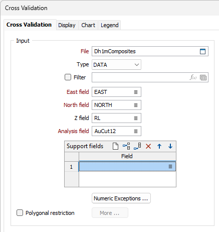
File
Double-click (or click on the Select icon) to select the name of the file containing the test dataset. The input file is normally the output file from Semi variograms.
East and North and Z fields
Specify the names of the fields in which Easting, Northing, and Reduced Level (Z) coordinates are stored in the input file.
If the input model is a 3D model, the Z field must be specified. If the input model is a 2D model, the Z field is optional.
Analysis field
Double-click (or click on the Select icon) to select the name of the field on which you want to perform the analysis.
Support fields
To support multivariate data for Co-kriging, specify one or more fields. These fields will be shown in the chart
Polygonal Restriction
Optionally, select the Polygonal Restriction option and click the More button to restrict which points are used in the estimates. For more details, refer to the Polygonal Restriction topic.
Numeric Exceptions
(Optionally) Use the Numeric Exceptions group to control the way that non-numeric values are handled. Non-numeric values include characters, blanks, and values preceded by a less than sign (<).
Output
Double-click (or click on the Select icons) to select the names of the Output files.
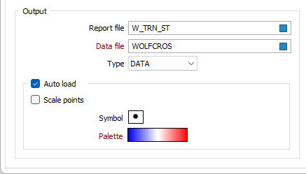
Report file
Once estimated values have been calculated for all points, they will be plotted in Vizex. Statistics relating to the data set are written to a (.RPT) Report file. The most important of these are the Mean Error Statistic and the Standard Deviation of the Error Statistic. If the model is exactly correct, these two values should be zero and one respectively. Changes to the model will be reflected in these values. There is no way of determining what are acceptable values in all circumstances.
When a log-normal (NATURAL LOG) transformation is selected, logarithmic values are written to the Report file along with the back-transformed logarithmic values and are not a direct replacement for the un-transformed values of the report.
No matter which transformation method is used, the application will always auto-load the points using the un-transformed or back-transformed SIZE field. You can however, switch to the LN_SIZE field if you prefer.
Data file
The Data File contains the coordinates of each point, the value in the Estimate and Residual fields for each point, and the Error statistics for each point.
Auto load
Select this check box to load the validated data as a Point layer. By default, the points in the display are coloured by ERROR STATISTIC. If a symbol and a palette are also applied to the data, this may further help to highlight any data values that differ markedly from their modelled values.
Scale points
Select this option to scale the displayed points by ERROR STATISTIC.
Symbol
A range of standard (Circle, Square, Diamond, Pentagon, Hexagon, Star, Triangle, Plus, Cross) marker symbols are available for selection in a drop-down list.
Palette
Double-click on the Palette box to choose a palette. You can also right-click on the box to see a preview of the current palette.
Model
Select an estimation model method and set modelling parameters:
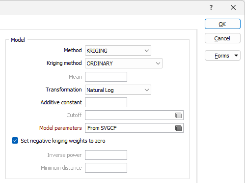
Method
Select an estimation method. See: The different estimation (gridding) methods for 2D block
Kriging method
When the Kriging method is set to SIMPLE, the global mean is assumed to be constant throughout the study area. If the Mean response is blank, the global mean is automatically calculated from the input data.
When the Kriging method set to ORDINARY, the local mean is recalculated each time the search neighbourhood is positioned on a new block centroid, but is kept constant within that neighbourhood.
Other Kriging methods are also available on the Block Model tab, in the Estimation group.
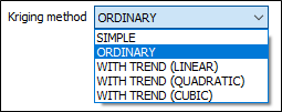
Trend
When the Kriging method is set to WITH TREND (also known as Universal kriging), the local mean within each search neighbourhood is modelled as a smoothly varying function of coordinates, rather than being held constant. The trend is usually modelled as a low-order polynomial function such as LINEAR (power 1), QUADRATIC (power 2), or CUBIC (power 3).
In an interpolation situation (estimating values at locations surrounded by input data), kriging with a trend offers no advantages over Ordinary Kriging and is disadvantaged through having to perform additional calculations. In an extrapolation situation (estimating values at locations beyond the input data), Universal Kriging may offer some advantages, but only if the physics of the phenomenon suggest the most appropriate trend model. Care is needed as the estimated values will depend very heavily on the chosen model (Goovaerts, 1997, p.152).
Local trend
Define the Local Trend of the data. This pertains to the scale of estimation.
Transformation
If you need to transform the data in the analysis field before the calculation, choose the appropriate transformation and enter the related parameters.
Aside from not altering the data at all, the most commonly-used transformations are NATURAL LOG and INDICATOR. See: Transformation
Additive constant
This input will be enabled if you have set Transformation to NATURAL LOGS.
Enter a value. This is the (calculated) amount that must be added to the raw data values in a sample, so that the natural logarithms of those values are normally distributed.
Cutoff value
This input will be enabled if you have set Transformation to INDICATOR.
Enter a value to define the maximum value that will be displayed on the graph. For example, if the cutoff value is set to 10 (gm) and a file contains grades ranging from 0-100 gm, all values in the ranges 10 to 100 gm will be displayed as though they had a value of 10 gm.
Model parameters
If you have chosen KRIGING as the Estimation method, right click in the Model parameters input box to enter azimuth and plunge values for the main, 2nd and 3rd directional variograms. To open the Semi Variogram Model form, right-click in the main, 2nd and 3rd direction input boxes. See: Model Type
Set negative kriging weights to zero
If you have chosen KRIGING as the Estimation method, select the "Set negative kriging weights to zero" check box to adjust the negative weights so that they have no effect. Since these zero weight samples are included in the count, the condition for the numbers of samples is met. You can do two runs with and without negative weights set to zero to see what the actual difference is.
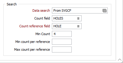
Search
Data search
Double-click to load a form set. Alternatively, right-click in the Data Search input box to open a form where you can define the shape and direction of the Search Ellipsoid Parameters.
The 3D (Plunge, Dip, and Thick Factor) parameters in the Data Search form will be disabled if a Z field is not specified.
Count field
Enter the name of a new field that will be used to store a Count of the number of values (in the nominated Count Reference field) used to calculate estimates.
Count Reference field
If you have specified a name for the Count field, then the Count Reference field input is enabled. Select a field from the sample or composite file (i.e. Hole_ID) which will be used as a reference counter.
Min Count field
Optionally, use the Min Count field to specify a minimum number of values to be applied to the calculation for each block.
Min & Max count per reference
In effect, the Min count per reference and Max count per reference values allow you to apply a filter condition. For example, you may want to ensure that, for every hole, you only count a certain number of "best" points.
- Min count per reference is useful when you want to specify that you only want holes that have a certain minimum representation in a search space (so that points are not counted, for example, when a particular hole has only one point in its search space).
- Max count per reference is useful when you want to specify that all the points found in a search space should not come from a single hole.
Both of these parameters use the Count Reference field to constrain the points that are selected by the grade interpolation process.
For Example:
If Min count per reference = 2, Max count per reference = 6, Maximum points per sector = 8, and the "Count reference field" = HOLE_ID, then, for each search space we want to find points to base our calculations on:
The process will look at that search space and only count points from holes where at least 2 points are present, only take the 6 "best points", and take a total of 8 points per sector (those 8 can be from any holes).
Forms
Click the Forms button to select and open a saved form set, or if a form set has been loaded, save the current form set.
Run
Finally, click Run to run the cross validation.