Interpolation Method
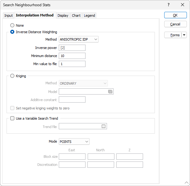
On the Interpolation Method tab of the Search Neighbourhood form, the option to apply an Inverse Distance Weighting or Kriging interpolation method is provided.
Inverse Distance Weighting
Select an estimation model method and the following modelling parameters:
Method
Choose either ANISOTROPIC IDP (the default) or INVDISTPOW as the estimation method. See: The different estimation (gridding) methods for 2D block
Inverse power
The weighting given to each point that falls within the search ellipse is inversely proportional to its distance from the block centre, raised to the value you enter in the Inverse power prompt.
Minimum distance
Enter the minimum distance between any sample point and the centre of the block being modelled. If true distance is less, the minimum distance value will be used instead. This method can eliminate the overpowering effect of samples very near to the block centre, but should not be used if the interpolation needs to honour the original data.
Min value to file
Specify the minimum value that will be written to the Input file.
Kriging
Select a Kriging method and the following modelling parameters:
Method
When the Kriging method is set to SIMPLE, the global mean is assumed to be constant throughout the study area. If the Mean response is blank, the global mean is automatically calculated from the input data.
When the Kriging method set to ORDINARY, the local mean is recalculated each time the search neighbourhood is positioned on a new block centroid, but is kept constant within that neighbourhood.
Other Kriging methods are also available on the Block Model tab, in the Estimation group.
Trend
When the Kriging method is set to WITH TREND (also known as Universal kriging), the local mean within each search neighbourhood is modelled as a smoothly varying function of coordinates, rather than being held constant. The trend is usually modelled as a low-order polynomial function such as LINEAR (power 1), QUADRATIC (power 2), or CUBIC (power 3).
In an interpolation situation (estimating values at locations surrounded by input data), kriging with a trend offers no advantages over Ordinary Kriging and is disadvantaged through having to perform additional calculations. In an extrapolation situation (estimating values at locations beyond the input data), Universal Kriging may offer some advantages, but only if the physics of the phenomenon suggest the most appropriate trend model. Care is needed as the estimated values will depend very heavily on the chosen model (Goovaerts, 1997, p.152).
Model
Double-click in the Model input box to load a form set. Alternatively, right-click to setup semi variogram model parameters. See: Semi Variogram Parameters
Additive constant
If you have chosen the NATURAL LOG Transformation option on the Input tab of the form, optionally specify an Additive constant to improve the fit between the data and a true log-normal distribution. The best way to determine the additive constant value is to display a histogram of your data (Stats | Histogram) and then click the 3 Parameter Log Normal button on the chart toolbar. Refer to Section 4.2 of Clark and Harper (2000) for more information on applying this correction.
Set negative kriging weights to zero
Select the "Set negative kriging weights to zero" check box to adjust the negative weights so that they have no effect. However, the zero-weight samples are still included in the search neighbourhood point count, ensuring that the conditions for minimum and maximum number of samples are met.
Negative kriging weights arise when points are very close, or when distant points are masked or screened by points closer to the block being interpolated. Negative weights are generally undesirable when estimating grades, and you would typically enable Set negative kriging weights to zero in this scenario.
Use a Variable Search Trend
Select this option to use a structural interpretation of the raw data to model the semi variogram.
Double-click (or click on the Select icon) to select a (*.mmstf) Trend file. The structural trend file you select here is an output of the Create Trend function on the Block Model tab, in the Variable Trend group.
If this option is selected, your attribute fields (above) will need to reference an omni-directional variogram created using the same trend model.
Mode
Select a (POINTS or BLOCKS) mode to calculate statistics for points or for blocks.
Select BLOCKS mode to calculate estimates for blocks, typically in ore estimation. Each block is the average of a series of points that are evenly distributed within the block. If BLOCKS mode is selected, specify the parameters for discretisation.