Gaussian Anamorphosis
![]()
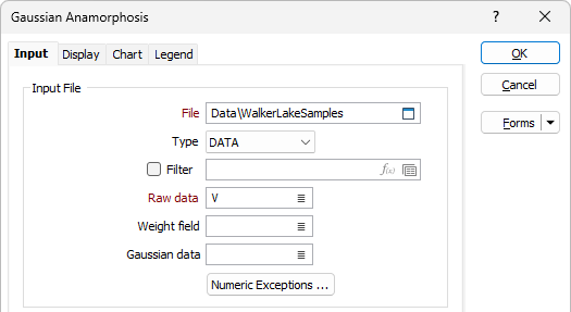
Input
Choose a file and associated raw data field, and optionally choose a weighting field.
Enter a Gaussian Data field name.
This option adds a column to the input file, which records the transformed Gaussian values of the samples in the raw data field. If you display this field in the Histogram, you will see a near-perfect normal distribution.
Hint: Although Gaussian numbers can have values anywhere between minus 5 and Plus 5, they most often fall between -3 and + 3.
(Optionally) Use the Numeric Exceptions group to control the way that non-numeric values are handled. Non-numeric values include characters, blanks, and values preceded by a less than sign (<).
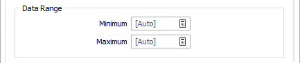
Data Range
Enter, or click the Auto Calculate icons to calculate, numeric values which define the lower and upper bounds of a data range. Entries should be based on your knowledge of the input data set.
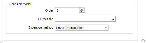
Gaussian Model
Enter a Gaussian Model output file name to store a binary version of the Gaussian model for later reuse.
Use the Order increment and decrement controls to control distortion so that the curve of the Gaussian distribution closely matches your data.
The same option is available on the Chart | Gaussian Anamorphosis tab when you run the chart.
The Inversion method drop down is used to select the method to be used to perform the gaussian variable transformation. The available methods are:
-
Linear Interpolation - Linear interpolation inversion uses a linear interpolation of the anamorphosis to calculate the inverse of the function. Points with identical Gaussian values are assigned the same raw values.
-
Linear Interpolation (Smooth) - Similar to Linear Interpolation except that points with identical Gaussian values are assigned different raw values to create a 'smoother' curve.
-
Frequency - This method computes raw values from the input Gaussian values directly and does not rely on the input Gaussian Model. The input Gaussian values are sorted by increasing order and a cumulative Gaussian distribution is fitted to their cumulative frequency. The cumulative Gaussian distribution is then used to compute raw values from the input Gaussian values. Points with the same Gaussian values are assigned different raw values - resulting in a perfect histogram where weights are not specified.
Click OK to display the chart.
The left-hand view displays the Gaussian values of the input data, along with the fit of the polynomial function. The right-hand side of the chart displays the histograms of the model (red) and raw data (blue).
The application uses Hermite polynomials to create a piecewise polynomial function that matches the raw data distribution. Use the spin control near the top of the chart to adjust the number of Hermite polynomials within the range of 1 and 200. However, because each increment adds complexity, you should aim for the smallest number of Hermite polynomials that fit the data.
Once you are satisfied with the fit of the polynomial, you can use the Gaussian data field like any normal variable.
If you make any changes to the Gaussian data field during Gaussian Anamorphosis Modelling, you must back-calculate it into real-world values. To do so, on the Stats tab, in the Transformation group, select Gaussian Anamorphosis | Back Calculation and supply the Gaussian data and Gaussian model, along with a name for the back-transformed data.