Open Pit Reserving Workflow

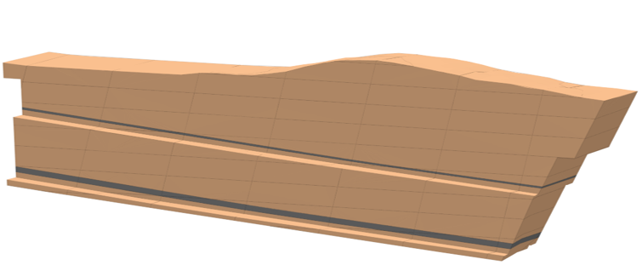
A Pit Solid is generated by running Create All Closed Volumes over the Pit Shell and the Topography.

To position an initial strip line, the Measure tool can be used against a reference layer:

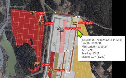
An initial strip line can then be drawn in Smart Snap mode, with Limits set for Distance, Bearing and Grade.

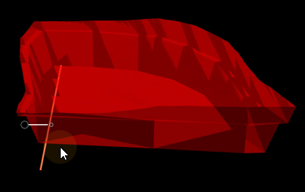
A starting Z value can also be determined by using Snap to Point on Segment to determine the lowest extents of the pit. The Move Z tool can then be used to adjust the Z level of the strip line accordingly. (The pit shell can be given some transparency to be able to see the line.)

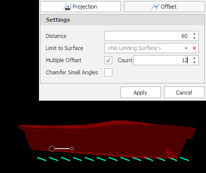
The Measure tool can also be used against a reference layer to determine an appropriate strip width, before the Offset tool is used (with the multiple offset option selected) to create strip lines running across the bottom of the pit. (A negative or positive offset distance value may be entered, depending on the direction in which the initial strip line was drawn. Alternatively, you can use the Reverse Sequence tool to reverse the direction of the strip line.)

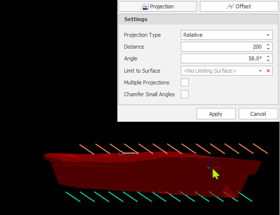
Once the strip lines have been offset, the Projection tool can be used to project the strip lines up to a Z level above the top of the pit.

To determine the parameters to apply to project the strip lines up to a Z level above the top of the pit, the Measure tool can be used in Smart Snap mode and with appropriate Limits set for Distance, Bearing and Grade.

In this example, the projection is not surface-limited. If a surface limitation is required, a structural boundary can be drawn based on available grid data. The Multi-line Relimit tool can then be used to ensure the strip lines fall within the boundaries of the grid.

Tip: In more complex scenarios, you can generate strip lines by applying a Projection Sequence. An existing sequence of offsets and projections can be selected and modified if required, or a new sequence can be created in the Projection Sequences Window, which is accessible from the Apply Projection Sequence tool or the Design | Setup right-click menu in the Project Explorer.

Once the strip lines are positioned and sized, the Set Attributes by Direction tool is used to increment a Strip attribute value, from West to East, for each strip line.

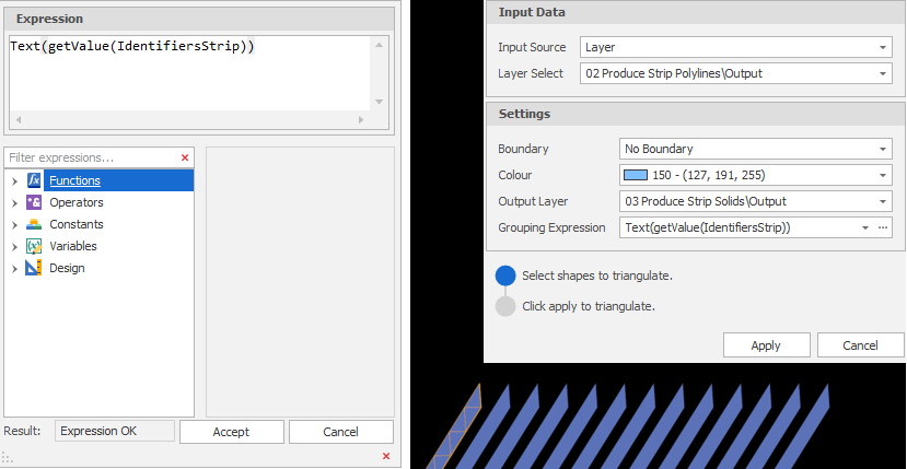
Once strip polylines have been attributed, offset and projected, the next step is to use the Create Triangulation tool to generate strip surfaces. The Strip attribute that was assigned to the strip lines is referenced in a Grouping Expression to create the surfaces.

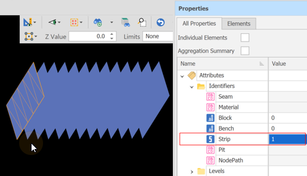
Since the strip surfaces do not inherit the Strip attribute values from the input strip lines, the Set Attributes by Direction tool is used once again to increment a Strip attribute value, from West to East, for each strip surface.

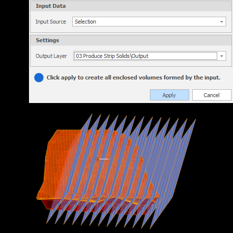
To cut the pit solid into strip solids, the pit solid and the strip surfaces are used as inputs to the Create All Closed Volumes tool:

Again, since the strip solids do not inherit the Strip attribute values from the input strip surfaces, the Set Attributes by Direction tool is used to increment a Strip attribute value for each strip solid:

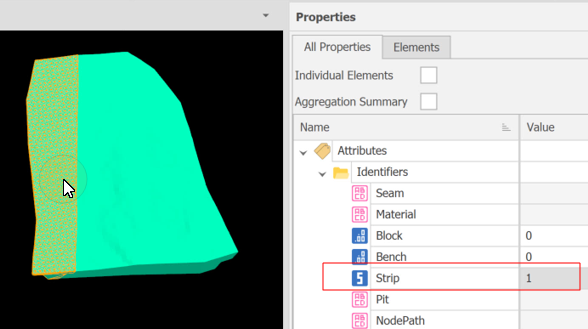
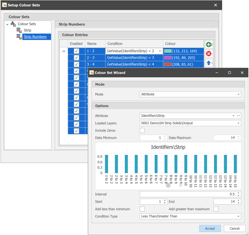
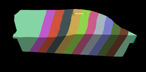
At this point, the Apply Colour Set tool and the Colour Set Wizard can be used to colour the strip surfaces by Strip attribute.

Strip solids are cut into blocks and benches using polygon block boundaries. The Measure tool is used against a reference layer to determine the distance and bearing required when drawing an initial boundary line:

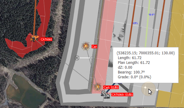
The Measure tool can also be used to determine the block size before boundary lines are created using the Offset tool (with the Multiple Offsets option selected).

To close-off the lines to create polygon block boundaries, the Create Shape tool is used with the Snapping mode set to Snap to Segment:

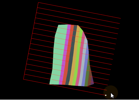
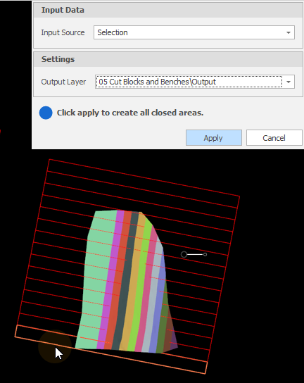
Once the block boundaries have been drawn, the next step is to convert the lines into closed polygons using the Create All Closed Areas tool:

The block polygons are then sequentially numbered with a Block number attribute from North to South using the Set Attributes by Direction tool.

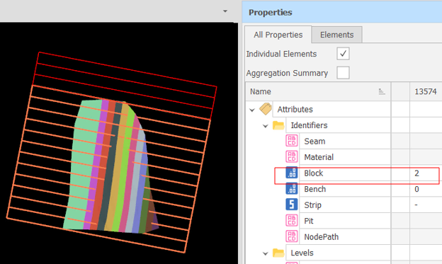
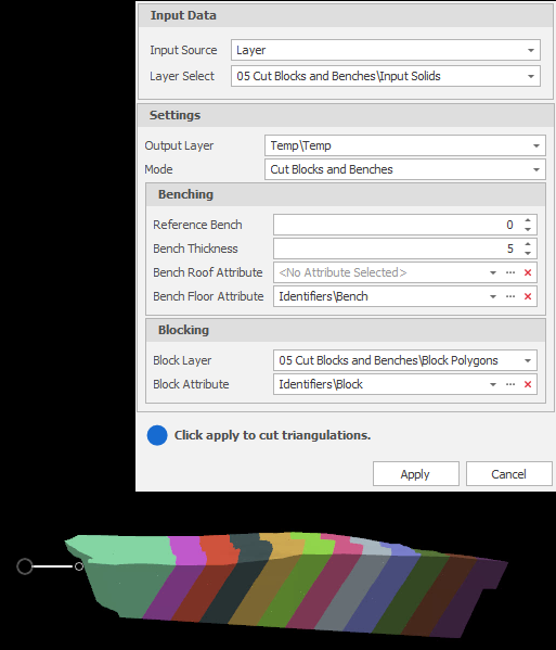
After using the Properties window to verify that the Block attribute has been populated for all of the block polygons, the strip solids and the block polygons are supplied as inputs to the Cut Blocks & Benches tool.

To cut the blocks and benches, a Bench Floor attribute (or a Bench Roof attribute or both) and the Block Attribute of the input block polygons are selected:

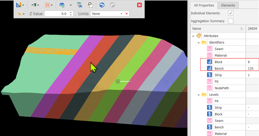
The Properties pane can be used to verify that Block and Bench attributes have been assigned:

Once Strip, Block and Bench solids have been cut, the final step is to Cut Stratigraphy into those solids.

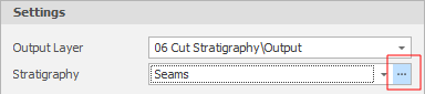
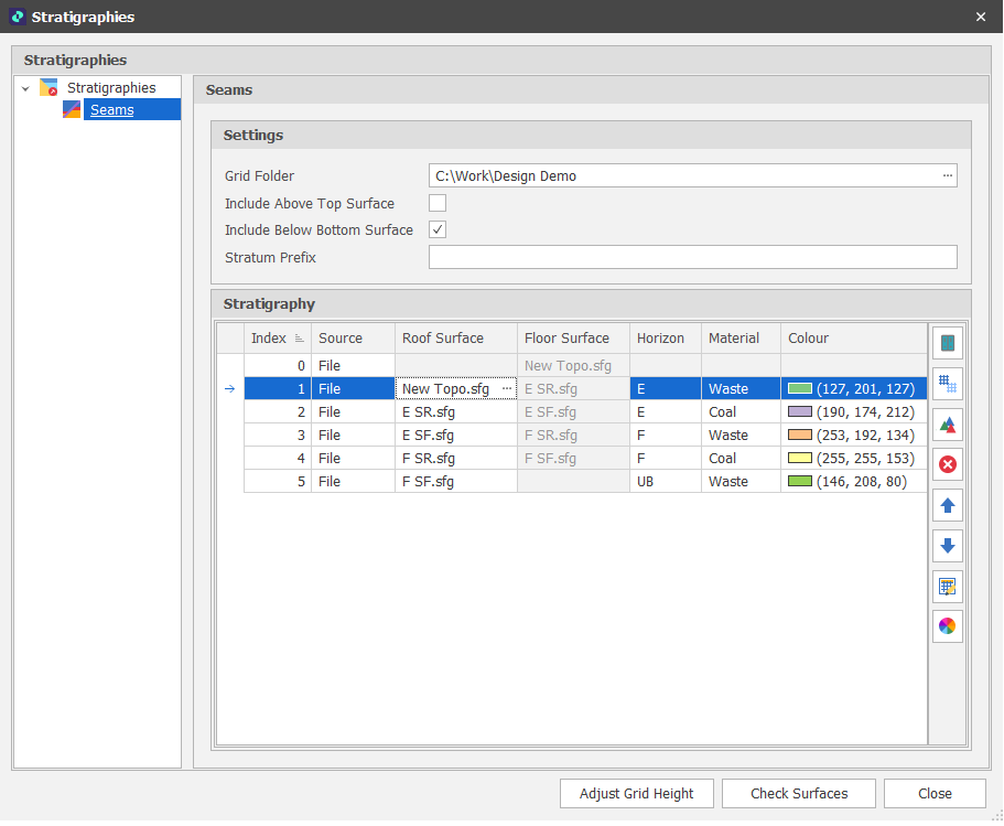
As a prerequisite, the Setup Stratigraphies utility is used to identify which seams or horizons are of interest, what their order is, which grids define their roof and floor, and which Horizon and Material attributes can be written to the stratigraphic solids at the time of cutting (typically, the name of each seam and whether the seam contains waste or ore material).

The Setup Stratigraphies utility is accessible from the Cut Stratigraphy tool and can also be accessed from the Design | Setup right-click menu in the Project Explorer.

In the following example, E SR, E SF, F SR and F SF are Grid files which represent the Roof and Floor of the seams that run through a pit. The layering of those seams and the materials they contain have been defined.

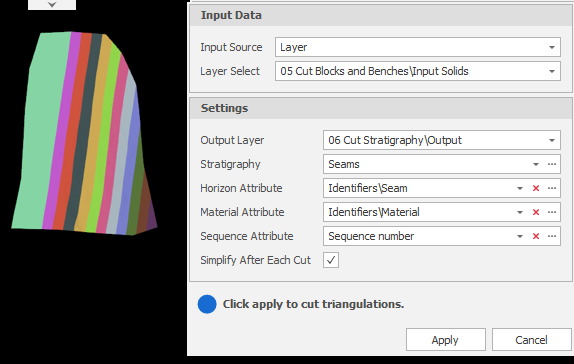
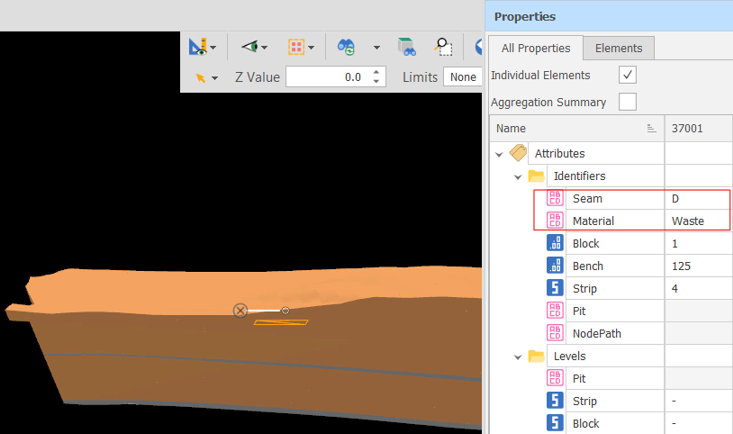
The Cut Stratigraphy function generates a new set of solids by cutting seams into the input solids. The Properties pane can be used to verify that the Horizon (Seam) and Material attribute values of the stratigraphy have been written to the new solids. Once Strip, Block, Bench and Stratigraphic solids have been cut, they can be loaded into a Data Table ready for Scheduling.

The Properties pane can be used to verify that Seam and Material attributes have been assigned:

Before (Strip, Block, Bench and Stratigraphic) design data can be written to a Data Table, a Volume attribute needs to be written to those solids. If Volume attributes do not already exist, they can be created using the Setup Attributes function, which is accessible from the Design | Setup right-click menu in the Project Explorer.

To write Volume attribute values to selected solids, the Set Attribute by Expression function is used. As the name suggests, an expression is used to calculate the volume of the selected solid or solids, for example:

GetSolidVolume(CurrentElement)

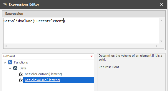
Tip: To save an expression for later re-use, in the Set Attribute by Expression dialog, you can set the expression method to Expression Sets, create an Expression Set called Calculate Volume, select the Volume attribute and enter the same expression.

You can manage Expression Sets from the Design | Setup right-click menu in the Project Explorer. For more information, see: Attribute Expression Sets

Now that we have Strip, Block, Bench and Stratigraphic (Seam) solids, we can go ahead and import them into the model database, however there are two prerequisites:

1. Right-click on the destination data table and choose Setup Levels to make sure that the table level hierarchy matches that of the model (typically, Pit, Strip, Bench, Block, Seam).

   

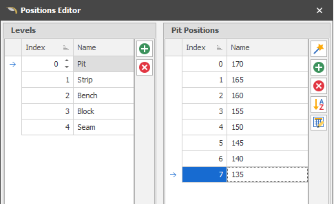
   Positions are created during the Import process. For more information, see: Levels

2. Having reconciled the levels, on the Home tab, in the Setup group: Select Fields to manage the fields that will be mapped to the attributes of the imported solids:

   For example:

   • Create a Qualities folder (this will be used to add Quality fields later).

   • Create an Imported folder with Waste and Coal subfolders.

   • Under the Waste folder, create a "Waste Solid" field of type Solid and also create a Volume field for waste.

   • Under the Coal folder, create a "Coal Solid" field of type Solid. Copy the Waste Volume field and paste it here to add a Volume field for coal.

3. Right-click on the destination data table and select Design Layers.

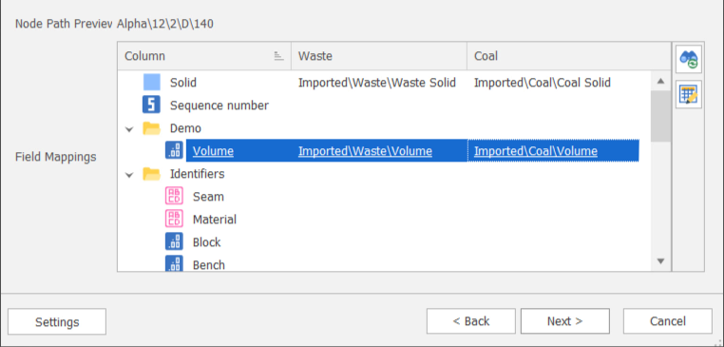
   As part of the Import process you will need to map the levels defined in the attributes of the solids with the levels defined in the table:

   

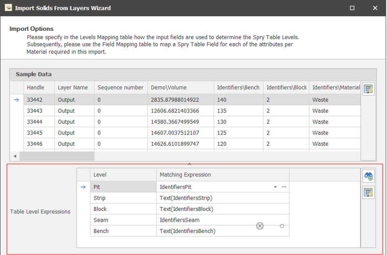
   And map the Coal and Waste Solids and Volume fields to the corresponding attributes of the imported solids:

Once the design solids and their volumes have been written to a data table, Qualities fields can be added to the table prior to those fields being populated with values calculated by sampling quality grids.

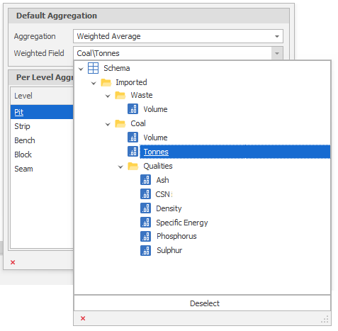
On the Home tab, in the Setup group: Select Fields to create Coal quality fields in the Qualities folder that was setup earlier and (if applicable) specify their aggregations. The quality fields that are added will match the qualities in the grid files that will be imported during Table Grid Sampling.

For example:

• You add a Tonnes field under the Coal folder as a calculated field: Coal Volume * Density

  This can then be used as the aggregation weighting field for other qualities that you add (Ash, CSN, Specific Energy, etc.) depending on the quality grids sampled.

• You set the Waste Volume, Coal Volume and Tonnes field aggregations as: Sum

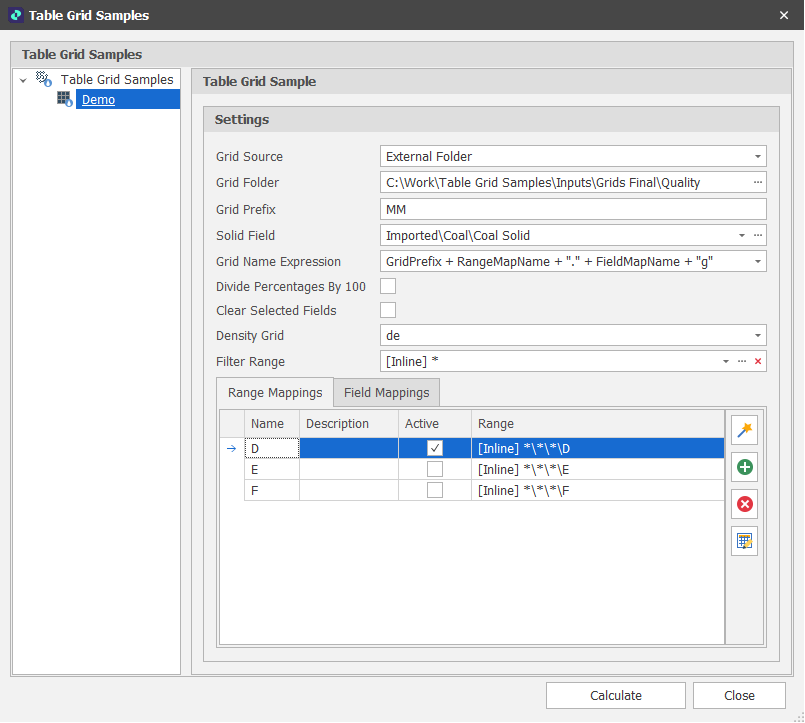
Once solids and volumes have been saved to the data table and their quality fields and aggregations defined, the Table Grid Samples function (available via when you right-click on a Table in the Project Explorer and select Setup | Table Grid Samples) is used to assign qualities based on the relationships between the solids and their associated quality grids.

At this point an imported section has been added to a Deposit Table. The example below shows a single strip in the animation, each solid represents a unique combination of Pit, Strip, Block, Bench, Seam and Material.