Options

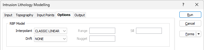
On the Options tab of the Intrusion Lithology Modelling form, set the parameters and define the surface area for the interpolation.

RBF Model

To generate a realistic implicit model, it is essential to restrict the effect of each drillhole sample to the surrounds of its local region. This is achieved using Interpolant functions which have similar options to variograms for range, sill, and nugget.

CLASSIC LINEAR	The standard linear kernel.
LINEAR	A linear kernel with an option for a nugget. The slope is defined by the ratio (Sill - Nugget) / Range, whilst the effect of the nugget is controlled by the ratio Nugget / Sill.
	Nugget is simulated by adding a small Gaussian component to the kernel, which has the tendency to produce more lumpy surfaces at each data point.

Using a non-zero nugget leads to longer processing times.

Drift

Drift determines how the value distribution is modelled further away from the sampled data:

NONE	The interpolant decays to zero.
CONSTANT	The interpolant assigns a constant value which is an approximation of the mean of the data.
LINEAR	The interpolant varies linearly.

Range

If you have chosen the LINEAR interpolant, enter a Range value.

The exponential variogram never reaches the sill. The range is the point where the variogram reaches 96% of its sill value.

Nugget

If you have chosen the LINEAR interpolant, enter a Nugget value. The Nugget value (effect) is the variance at distance zero. This is always less than the sill. The nugget effect arises because the regionalised variable is erratic over a very short distance that that the semi variogram goes from zero to the nugget effect in a distance less than the sampling interval.

Sill

If you have chosen the LINEAR interpolant, enter the Y coordinate (semi variogram) value of the sill for each component of the model. This is constant for a dataset.

Points/Sphere

In most cases it is impractical to create a single model using all the points in the data set. Instead, the data set can be divided into overlapping regions. These regions are defined by the direction of propagation of spheres across the input data:

The Points/Sphere value is the number of points you want to look at per sphere. The radius of each sphere will therefore depend on the concentration and the distribution of the points in the input data.

This value is calculated automatically based upon the input data. Unless a number is entered, the field defaults to [Auto].

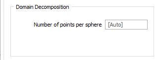
Domain Decomposition

In most cases it is impractical to create a single model using all the points in the data set. Instead, the data set can be divided into overlapping regions. These regions are defined by the direction of propagation of spheres across the input data:

The Number of points per sphere is the number of points you want to look at per sphere. The radius of each sphere will therefore depend on the concentration and the distribution of the points in the input data.

This value is calculated automatically based upon the input data. Unless a number is entered, the field defaults to [Auto].

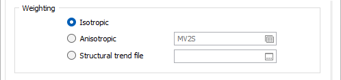
Weighting

Select a Weighting option:

• When you select an Isotropic orientation method, there is no preferred direction.
• When you select an Anisotropic orientation method, you enter a preferred direction, as well as specify the weighting in that direction.

Double-click to load an existing form set. Alternatively, right-click in the Anisotropic input box to open a form where you can define the shape and direction of the search ellipsoid.

The ability to apply a weighting based on the orientation of a data search ellipsoid is a useful option. Although it references the same set of parameters used to define a data search for block modelling, only a few of the values are utilised by implicit modelling.

For example, only the factors and rotation associated with the orientation axes are used – the radius is ignored and will be greyed out. If you consider that there is a greater correlation in one direction in particular, select Ellipsoidal, and set appropriate factor, azimuth, plunge and rotation values.

This effectively accounts for any anisotropy. Interpolation weights can be adjusted accordingly; data points located along the major semi-axis will receive a higher weighting than those located along the minor semi-axis, for similar distances from the prediction location.

• When you select Structural Trend File, a data search weighting is derived from the direction of anisotropy defined in a (*.mmstf) Structural Trend File, which is an output of the Implicit Modelling | Structural Trend | Create Trend function.

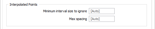
Interpolated Points

Minimum interval size to ignore

The Minimum interval size to ignore is auto calculated as a fraction of the median interval length for included and excluded intervals.

This will put the first positive point at the minimum interval size/2 from the boundary when creating negative and positive points. This will also ignore intervals smaller than the interval size.

Accept the default [Auto] or specify the minimum length interval you want to be included in the lithology model. If this value is too high, some small intervals may not be included in the interpretation. If the value is too low, small intervals, which may create small stand-alone blobs, may be included in the interpretation.

It may be useful to generate interpolated points, if adjusting the weighting preferred direction does not give you a wireframe that is geologically valid. This will often help explain how the wireframe was created. These points can be edited, or you can add points to the file to modify the way the wireframe will be created. These points can then be interpolated using Implicit | Surface | Attributed Points. See: Attributed Points

Maximum Spacing

The Maximum spacing is auto calculated per drillhole interval, based on the distance to the closest interval of an opposite INCLUDED/EXCLUDED status.

Accept the default [Auto] or specify the Maximum Spacing (in grid units) that will be used to position the points relative to each interval. Choose a number that fills in the big intervals. You don’t want it to be too small because this will add unnecessary complexity to the interpolator. However, you do want the big intervals to have more than two offset points.

Try to strike a balance. Is the spacing too low (too many points give you information that isn’t useful) or is the spacing too high (big intervals with long regions without any points).

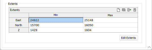
Extents

Define the area of interpolation:

East, North and Z fields

Specify the Minimum and Maximum extents of the surface in the East, North and Z directions.

Edit Extents

Click the Edit Extents button to collapse the form and visually adjust the extents, automatically aligning the extents to a restriction rectangle in Vizex. Interactively adjusting the extents rectangle in the Vizex display, or in the Vizex Property Window, will update the values in the form.

Output

See: Edit Extents