Modelling Parameters

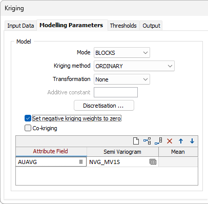
On the Modelling Parameters tab of the Kriging form, select a Mode, a Kriging method, and specify the number of divisions for Discretisation. You can also apply a Trend and select a Transformation.

Model

Mode

Select a (POINTS, BLOCKS or POLYGONS) Kriging mode and specify the parameters for discretisation. Discretisation is only available when BLOCKS or POLYGONS mode is selected.

Method

When the Kriging method is set to SIMPLE, the global mean is assumed to be constant throughout the study area. If the Mean response is blank, the global mean is automatically calculated from the input data.

When the Kriging method set to ORDINARY, the local mean is recalculated each time the search neighbourhood is positioned on a new block centroid, but is kept constant within that neighbourhood.

Other Kriging methods are also available on the Block Model tab, in the Estimation group.

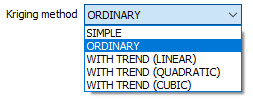
Trend

When the Kriging method is set to WITH TREND (also known as Universal kriging), the local mean within each search neighbourhood is modelled as a smoothly varying function of coordinates, rather than being held constant. The trend is usually modelled as a low-order polynomial function such as LINEAR (power 1), QUADRATIC (power 2), or CUBIC (power 3).

In an interpolation situation (estimating values at locations surrounded by input data), kriging with a trend offers no advantages over Ordinary Kriging and is disadvantaged through having to perform additional calculations. In an extrapolation situation (estimating values at locations beyond the input data), Universal Kriging may offer some advantages, but only if the physics of the phenomenon suggest the most appropriate trend model. Care is needed as the estimated values will depend very heavily on the chosen model (Goovaerts, 1997, p.152).

Transformation

Select the method that will be used to process the data before it is used by the function:

• NONE – For normally distributed data. Uses the raw data values. This is the default.
• NATURAL LOG – For log-normally distributed or positively skewed data (such as precious metal assays).

Additive constant

If you have chosen NATURAL LOG, optionally specify an Additive constant to improve the fit between the data and a true log-normal distribution. The best way to determine the additive constant value is to display a histogram of your data (Stats | Histogram) and then click the 3 Parameter Log Normal button on the chart toolbar. Refer to Section 4.2 of Clark and Harper (2000) for more information on applying this correction.

Parameters

Select the parameter set of the associated Model type to use in the calculation. Press F4 (or right-click | Edit) to create a new set. Press F3 (or double-click) to select an existing set.

Discretisation

Click on the Discretisation button to specify the number of divisions in the East, North, and Z directions. These are integer values that control the number of discrete points to be estimated in each direction within each block (or sub-block). The values of all the discretised points are then averaged to estimate the value for the block, and the result of each block is written to the output file.

For example, if you choose 4 East divisions, 4 North divisions, and 4 Z divisions, the application will interpolate and average a total of 64 estimates within each block. Although the estimates for a given block all share the same input data, the distance from each input sample (and thus the weight) will be slightly different for each discretised point, producing a different result for each one. The result is a more accurate estimate, but at the cost of more computing time. See: Discretisation

Set negative kriging weights to zero

Select the "Set negative kriging weights to zero" check box to adjust the negative weights so that they have no effect. However, the zero-weight samples are still included in the search neighbourhood point count, ensuring that the conditions for minimum and maximum number of samples are met.

Negative kriging weights arise when points are very close, or when distant points are masked or screened by points closer to the block being interpolated. Negative weights are generally undesirable when estimating grades, and you would typically enable Set negative kriging weights to zero in this scenario.

Alternatively, if you are using point data to model a tangible surface such as the elevation of a coal seam, including negative weights may improve the result.

Use the verbose reporting options when setting up the Kriging runs to find out what proportion of negative weights you have with your Kriging plan. If you have many blocks with negative weights, you probably need to adjust the search/sample number parameters you have set.

Co-kriging

Select this check box to run Kriging in Co-kriging mode.

When the check box is selected, the first attribute field listed (See “Attribute fields” below) is the only estimation field. All other fields are used to support Co-kriging.

Attribute fields

Additional attribute fields (and semi variograms) may be specified for multi-element interpolation, or for Co-kriging when that option is selected. Typically, these will be elements which correlate closely within the domain being interpolated. Use the buttons on the local toolbar to Manage the rows in the list.

The search conditions are applied to the primary attribute. This determines the group of records that will be used to estimate ALL attributes. It means that the results for secondary attributes may differ from those obtained had they been estimated separately.

This may occur when there are missing values, and when additional records are needed to satisfy the maximum number of search points.

Only the grades and weights of the first (primary) attribute are written to the verbose report file.

You can use an expression to fill the Attribute field value. Right-click and select Edit Expression to open the Expression Editor and build the expression.

Note: When expressions are used to select an attribute, the ability to name output fields using, or building upon, the name of the input attribute is lost because the implicit name becomes a part of the expression. In this instance when an Output field is required, a prompt will be displayed in which you can enter the name of the Output field: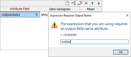

For detailed information on specifying output fields when using expressions, see Output Field Name Attributes.

Semi Variogram

Double-click in the grid or right-click on the Forms icon to set semi variogram model parameters.

A semi variogram model is said to have anisotropy if the range of the semi variogram differs with direction. The anisotropy defines the way that the Kriging weights are applied. It does not affect the way the modelling process searches for data.

If you have selected Use a Variable Search Trend as you Search option (below) your attribute fields will need to reference an omni-directional variogram created using the same trend model.

Mean

When the kriging method is set to SIMPLE, the global mean is assumed to be constant throughout the study area. If the Mean response is blank, the global mean is automatically calculated from the input data.

Search

Double-click to load a Data Search form set. Alternatively, right-click in the input box to open a form where you can define the shape and direction of the search ellipsoid. See: Search Definition

Search method

Use the Search method drop down to select the required search method for the data search - Legacy or Improved.

With the addition of new fields in Micromine Origin & Beyond v25.0, a new and improved data search algorithm was created. The order of the named sectors for Octant and Quadrant search ellipsoids has also been modified to a Z-order in the improved Search algorithm, making it easier to know which sectors are opposite.

The new algorithm aims to minimise the average distance from the ellipse centre, while maximising the number of included points (subject to the constraints). If the new fields are not used, the old algorithm is used so that users do not get unexpected or different results. The Improved option will utilise the new algorithm, which is more flexible than the Legacy one, so even with the same parameters, it can find more and/or slightly different point sets.

If you hover on a populated Data Search field, a pop up will display information on the parameters set for the selected search:

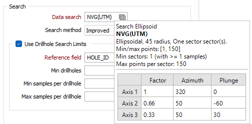
Use Drillhole Search Limits

Select the option to enable the options for the sector search parameters.

Reference field

Select a field from the sample or composite file (i.e. Hole_ID) which will be used as a reference counter.

Min drillholes

Optionally, use the Min drillholes field to specify a minimum number of drillholes to be included in the search.

Min & Max samples per drillhole

In effect, the Min samples per drillhole and Max samples per drillhole values allow you to apply a filter condition. For example, you may want to ensure that, for every hole, you only count a certain number of "best" points.

• Min samples per drillhole is useful when you want to specify that you only want holes that have a certain minimum representation in a search neighbourhood (so that points are not counted, for example, when a hole has only one point in its search neighbourhood).
• Max samples per drillhole is useful when you want to specify that all the points found in a search neighbourhood should not come from a single hole.

Both parameters use the Reference field to constrain the drillholes that are selected by the interpolation process.

FOR EXAMPLE:

If Min samples per drillhole = 2, Max samples per drillhole = 6, Maximum samples per drillhole = 8, and the Reference field = HOLE_ID, then, for each search neighbourhood we want to find drillholes to base our calculations on:

The process will look at that search neighbourhood and only count from holes where at least 2 samples are present, only take the 6 "best samples", and take a total of 8 samples per sector (those 8 can be from any holes).

Note that if the Maximum samples per sector is left blank, the maximum value will default to 150. If you want to allow for more samples, you need to explicitly enter a larger upper limit. The higher the upper limit, the slower the process will be.

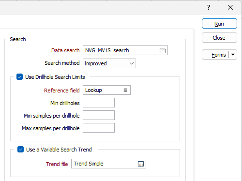
Use a Variable Search Trend

Select this option to use a structural interpretation of the raw data to model the semi variogram.

Double-click (or click on the Select icon) to select a (*.mmstf) Trend file. The structural trend file you select here is an output of the Create Trend function on the Block Model tab, in the Variable Trend group.

If this option is selected, your attribute fields (above) will need to reference an omni-directional variogram created using the same trend model.

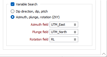
Variable Search

Select the Variable Search check box option to specify fields that contain variable values defining the rotation angles for the search ellipsoid, for each block in the file.

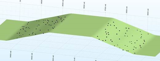
Where there is a significant directional variation in the continuity of the modelled mineralisation (in a folded structure for example) the Variable search option allows the rotation angles for the search ellipsoid to be defined. The search ellipsoid orientation can be controlled on a block-by-block basis, reflecting the directional trends in the mineralisation.

If you select the Dip Direction, Dip, Pitch option, you can select the fields containing these values for the variable search.

If you select the Azimuth, Plung, Rotation (ZXY) option, the Azimuth, Plunge and Rotation fields (for ZXY) can be specified.

These fields change the orientation of the variogram model as well as the search ellipsoid. Another way to think of it is that the variogram model axes are always aligned with the search ellipsoid axes.

If they are specified, the process will use the values in these fields rather than those defined in the Ellipsoid Parameters tab of the Data Search form.

If variable values in the block model file are missing, then the values defined in the Ellipsoid Properties tab will be used instead.

The Variable Search option can improve interpolation results for gently folded ore bodies. For data preparation prior to interpolation, the Flattening and Unfolding tools available in the application provide a more complex (yet more accurate) alternative.

Thresholds