Implicit Modelling
The traditional method of explicitly defining 3D geological or grade boundaries relies heavily on the time-consuming creation of surfaces or solids that are based on digitised strings or points. Implicit modelling is an alternative to explicit modelling which relies on a volume function.
This volume function can be used to construct models to represent grade, lithology or a geological surface in 3D, and takes away the need for time-consuming string or point digitising. Thus, the advantage of implicit modelling is that it is quicker and at times it may be better than trying to digitise complex geology. Implicit modelling may also help geologists see trends in the geological data and pick up faults or folds etc.
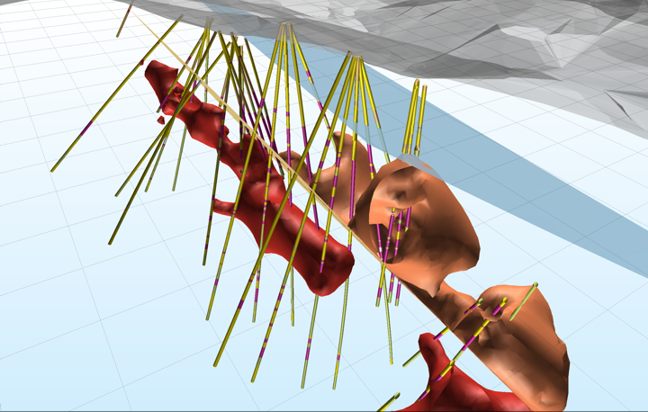
A faulted orebody created using the application’s Implicit Modelling module. The orebody is terminated by the semi-transparent blue fault at the top and is displaced by the pale fault at the centre.
Implicit modelling works on both closely drilled and sparsely drilled data, or a combination of both. It will also work well on data that is not systematically drilled (which may be hard to model using explicit modelling methods).
The application uses a volume function called Radial Basis Function (RBF) to model grade, volumes, and surfaces in 3D space.
Simple functions that can be used to generate surfaces and solids are available on the Implicit menu. A deep understanding of geostatistics, or of explicit modelling techniques, is not needed in order to use them.
- Implicit | Numerical | Grade is used to generate wireframes representing grade shells. The input data are typically composited drillhole assay values. See: Grade
- Implicit | Lithology | Intrusion is used to generate a wireframe representing the extents of lithology units, based on downhole logging information. See: Intrusion
- Implicit | Lithology | Contact is used to generate a wireframe representing the extents of lithology surface contacts or sheeted veins. See: Contact
- Implicit | Lithology | Vein is used to generate a wireframe representing the extents of lithology units, based on downhole logging information. See: Intrusion
- Implicit | Lithology | Fault is used to generate fault surfaces based on 3D points and/or strings (this data may include dip and dip direction). The Generate Fault algorithm should only be used with a small amount of points (< 500). See: Fault
- Implicit | Lithology | Geology is used to generate a full and accurate geological model, define the geological order and automate the boolean process based on the geological history, as well as model lithologies. See: Input
- Implicit | Lithology | Surface Map is used to generate wireframes and/or solids from surface map data such as boundary strings and structural measurements. See: Surface Map
- Implicit | Surface | Polygon uses an RBF (Radial Basis Function) to interpolate data from closed strings or polygons. See: Polygon
- Implicit | Surface | Point Cloud is used to create a surface using points resting on an open or solid surface. The output is a wireframe of that surface. See: Point Cloud
- Implicit | Surface | Surface Points is used to interpolate the points on a regular grid. A Points file, a Grid file, and a Wireframe can be generated from the interpolated data. See: Surface Points
- Implicit | Surface | Downsample Points is used to reduce the number of data points in an input dataset whilst retaining the integrity of the data. This is a pre-processing step for dense (e.g. LIDAR) data sets. See: Downsample
- Implicit | Surface | Attributed Points is used to create a solid from points that are output (and then perhaps edited) from the Modelling | Implicit Modelling | Lithology function. This function can be used to model any drillhole point data that contains positive and negative values. See: Attributed Points
- Implicit | Tools | Output Implicit Model is used to generate different output triangulations or points for the same model, without having to recompute the model each time. See: Output Implicit Model
- Implicit | Structural Trend | Create Trend is used to create a locally varying anisotropic model based on a surface. See: Create Structural Trend
- Implicit | Structural Trend | Display Trend is used to load a locally varying anisotropic model based on a surface. See: Display Trend
Terminology
For most users, the term “surface” is associated with an area (a DTM or a Grid), while “solids” have a volume. In the strictest sense a solid can be considered as a closed surface. All solids have an outer surface and any point (not exactly on that surface) lies either inside or outside that surface.
In the context of Implicit Modelling, the term “surface” is used in the more generic sense described above. Implicit Modelling is an indirect method of defining a surface. In simple terms, all points “outside” the surface are given a positive value and those “inside” are given a negative value. Within the spatial extents of the data, the surface of interest can be considered as the zero “contour”. Effectively the definition of this surface is based on a mathematical equation. It is “smooth” in the sense that the position of any point on the surface can be calculated exactly. Compare this to a gridded surface, where only the cell centres have a known value.
Processing
Each Implicit Modelling function is typically a two stage process. Firstly, a surface is generated using indirect methods. Secondly, the implicit surface is converted to a wireframe. Both stages require the user to define the following parameters.
Domain Decomposition
When doing any implicit modelling in the application, a surface or a solid is created. This open or solid surface is created from a point cloud using Domain Decomposition. Domain Decomposition is a continuous 3D function which is positive on one side of the surface and negative on the other. The zero-set of the function defines a surface or that smoothly interpolates between the input surface points.
In most cases it is impractical to create a single model using all the points in the data set. Instead, the data set can be divided into overlapping regions. These regions are defined by the direction of propagation of spheres across the input data:
The Number of points per sphere is the number of points you want to look at per sphere. The radius of each sphere will therefore depend on the concentration and the distribution of the points in the input data.
This value is calculated automatically based upon the input data. Unless a number is entered, the field defaults to [Auto].
Weighting
The ability to apply a weighting based on the orientation of a data search ellipsoid is a useful option. Although it references the same set of parameters used to define a data search for block modelling, only a few of the values are utilised by implicit modelling.
For example, only the factors and rotation associated with the orientation axes are used – the radius is ignored and will be greyed out. If you consider that there is a greater correlation in one direction in particular, select Ellipsoidal, and set appropriate factor, azimuth, plunge and rotation values.
This effectively accounts for any anisotropy. Interpolation weights can be adjusted accordingly; data points located along the major semi-axis will receive a higher weighting than those located along the minor semi-axis, for similar distances from the prediction location.
A data search weighting may also be derived from the direction of anisotropy defined in a Structural Trend File, which is an output of the Implicit | Structural Trend | Create Trend function.
Number of neighbours
This parameter is used in Point Cloud modelling to control local orientation of the modelled surface. In particular it is used to define the direction perpendicular to the surface. In other words it determines what is the “top” and “bottom” of the surface at any location. A minimum of 4 points are required for this calculation.
Try starting between 6 (sparse) and 20 (dense).
Output Wireframe Tolerance
A tolerance is specified in Grid units.
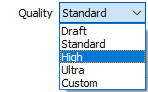
Quality
This setting provides a convenient way to control the quality and the speed of wireframe generation. There are five quality settings: Draft, Standard, High, Ultra and Custom.
Setting the quality to Draft allows the general shape of the output wireframes to be generated quickly.
With the exception of Custom, each quality setting has a pre-set error tolerance value. The error tolerance for Draft is approximately twice that for Standard, which, in turn, is twice that for High, etc.
Setting the Quality to Custom allows a user-specified error tolerance. There is no limit to the user-specified error tolerance value (and hence the minimum mesh size), other than that imposed by available system memory.
Max triangle Size
To eliminate large meshes, specify a Maximum Triangle Size parameter in grid units.
By default, mesh size is controlled by the tolerance parameter, which specifies the maximum error between the rendered surface and the actual surface. Typically, larger meshes are used where the surface is relatively flat, and smaller meshes are used where the surface has high curvature.
If a Max Triangle Size is specified then all triangles will be that size, or smaller if they fail the tolerance test.