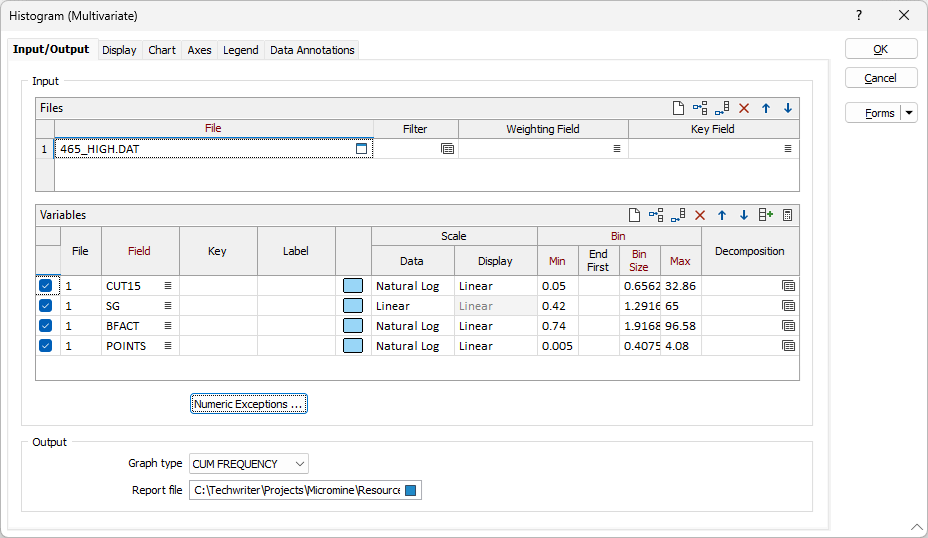
Histogram (Multivariate)
![]()
To generate distribution statistics for a single field, or for multiple fields using a different form set for each field, see Histogram.
Input/Output
Files
On each row of the grid, double-click (or click on the Select icon) to select the name of the files containing the source values. If required, define a filter to selectively control which records to process in each file.
Weighting field
For each input file, optionally select a Weighting field. When a Weighting field is applied, weighted means, standard deviations, confidence intervals and variances will be written to the report file. If no Weighting field is specified, un-weighted values will be written to the report file.
Key field
For each input file, optionally select a Key field (for example, a field that contains lithology codes or horizons) to create a plot for the unique values in that field. The plot names are formatted using the field name and each key value.
Note that default labels in charts often use the input field name to label the data being plotted. If these fields are expressions, then the expressions will be used as the label text. To avoid this, you can use an additional attribute to define the label. See: Output Field Name Attributes
Variables
Use the Variables grid list to specify the fields you want to generate distribution statistics for. Use the check boxes to choose which variables to include or exclude from the chart.
You can specify a display colour and a label for each field. Use the buttons on the local toolbar to Manage the rows in the list.
To create vertical labels, you can set the angle of the text to 90 degrees in the Advanced Axes Options. See: Advanced
Field
On each row of the grid, double-click (or click on the List icon) to select the field you want to generate distribution statistics for.
It is possible to use the autofill button on the grid toolbar to populate a new row by choosing a saved Stats | Histogram (univariate) form set. The univariate input file and the multivariate input files must be the same.
If the univariate histogram is set to autofit the ranges, then they will be calculated with the number of bins in the form.
Scale
For each variable, choose Scale options for the data and the display. The available options are:
- LINEAR When this option is chosen, the actual values in the Graph field are used subject to the settings in Numeric Exceptions.
- NATURAL LOG When this option is chosen, the values in the Graph field are converted into their natural logarithm. In this case, the minimum data value specified by the graph minimum must be greater than zero (since the Ln of zero is - infinity).
Bin
Minimum
Enter the minimum value that will be shown on the graph. The minimum value must be greater than zero.
If the Scale (Display) option has been set to NATURAL LOG (Ln):
- Enter the natural log value for the start of the graph.
End first bin
Enter a numeric value to define the end (upper limit) of the first bin on the display.
If the Scale (Display) option has been set to NATURAL LOG (Ln):
- Enter the natural log value that defines the upper limit of the first bin.
Bin size
If the Scale (Display) option has been set to NORMAL:
- The bin size defines the interval between successive increments (the width of the bars) on the graph. If, for example, the bin size is set to 0.1 (with the first bin ending at 0.05), the boundaries will be at 0.15, 0.25, 0.35 and so on.
- For detailed analysis, aim for around 50 bins. One rule of thumb for choosing the best bin size is to measure the range of the data (subtract the minimum value from the maximum value) and divide the result by 50. You may then use that value or round it to a simpler number.
If the Scale (Display) option has been set to NATURAL LOG (Ln):
- This input describes the size of each of the bins in the graph in terms of natural logs.
- Note natural logs (Ln) are logs to the base e. There may be up to 500 bins. Enter a value or click the Calculate button to calculate a bin size based on the other inputs.
Note: You can click the Calculate button on the grid toolbar (or right-click and select Auto Calculate) to generate a bin size based on the other inputs.
Maximum
If the Scale (Display) option has been set to NORMAL:
- Enter the maximum value that will be shown on the graph.
- If you use the short cut method (double click or F3) to obtain a value, it will be adjusted automatically to ensure there is an integer number of bins.
If the Scale (Display) option has been set to NATURAL LOG (Ln):
- Enter the natural log of the maximum value that will be displayed on the graph.
Decomposition
Decomposition attempts to reveal the underlying populations of data when the sample under investigation is composed of data drawn from a series of normally or log-normally distributed populations.
Click on the icon to load a saved form set, edit a saved form set, or create a new form set.
Numeric Exceptions
(Optionally) Use the Numeric Exceptions group to control the way that non-numeric values are handled. Non-numeric values include characters, blanks, and values preceded by a less than sign (<).
Output
Graph type
Choose a graph type (HISTOGRAM, CUM FREQUENCY, PROBABILITY PLOT) from the drop-down list.
Note that the Probability Plot graph type is a rotated chart. The x-axis is vertical, and the y-axis is horizontal. These axes are deliberately flipped so that x-axis always matches with the grade axis (as per the normal Histogram mode).
Scale
Choose a Scale option from the drop down list. The available options are:
- LINEAR When this option is chosen, the actual values in the Graph field are used subject to the settings in Numeric Exceptions.
- NATURAL LOG When this option is chosen, the values in the Graph field are converted into their natural logarithm. In this case, the minimum data value specified by the graph minimum must be greater than zero (since the Ln of zero is - infinity).
Report file
Enter (double-click or click on the Select icon) to select the name of the Report File that will be written as a result of the process. To see the contents of the file, right-click in the file box and select View (F8).
The Report Viewer is opened for any Statistical function that generates a Report file. Click the Form button on the Viewer toolbar to re-open the form, adjust the parameters of the Statistical calculation, and then choose to overwrite or append to the output in the Viewer window.
OK
Finally, click OK to run the function using the current parameters. There may be a short delay before the chart appears, depending on the amount of data to process. A progress bar will be shown at the bottom of the screen.