Solver
The production schedule is optimised using a mathematically proven Mixed Integer Programming (MIP) solver. Running the optimisation process will define which blocks should be mined in which period, to achieve the objective. On completion, the Mining Period attribute for each task is populated and a Start date and Finish date are calculated.
These dates indicate a possible mining sequence, based on the period and the horizontal, vertical and stage dependencies. By doing this, the tasks can be animated to give a realistic indication of what the mine will look like at any future date.
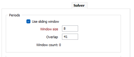
Periods
Use sliding window
The built-in solver has the option of defining a sliding window. This breaks the problem into smaller, overlapping time horizons in order to reduce the solution time.
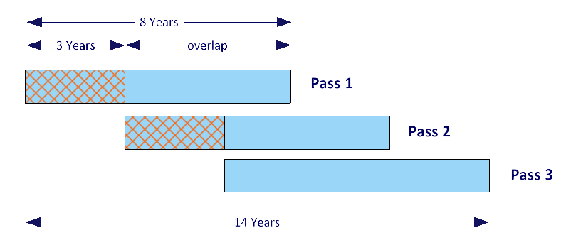
For example:
If the time horizon is 14 years, then choosing to use an 8 year sliding window with a 5 year overlap, will reduce the problem into 3 smaller parts. The first “pass” will consider all mining blocks, using a time horizon of 8 years. This solution will determine the blocks mined in the first 3 years (Window size - Overlap).
The second “pass” will exclude these blocks from the problem and this solution will determine the blocks to be mined in years 4 to 6.
The final pass will solve for years 7 to 14.
In practice, the solution obtained using sensible sliding window values will not be significantly different to the solution for all mining blocks across the complete time horizon. However, the performance gains can be significant. Considering the example above, common sense suggests that knowing which blocks will be mined in years 9 to 14 will have little effect on the blocks mined in years 1 to 3.
Input Filtering
Maximum split duration (days)
If you select the check box and enter a value in the Maximum task split duration (days) field, all tasks that are longer than the term duration are internally divided into "splits" of the term duration and no longer. The solver assigns periods to each split separately, allowing tasks to be scheduled across periods. the default value for the field is [Auto], and the period duration specified on the Optimise tab is used.
Splits created for a single task form a dependency chain - that is, each split must be mined in order and cannot occur after the following split. The decision to mine a task or not is still made for each entire task: either all splits from a task are mined, or none are. For example: If there are two tasks, t1 and t2 with a dependency from t1 > t2, then the first split from t2 depends on (must not be mined before) the last split from t1.
When quantities are reported for periods, quantities are accumulated by splits; if a task is split across periods, its quantity values are partitioned across periods according to the total split durations assigned to each period.
Note: Task splitting is internal to the optimisation process: Actual tasks in the schedule are not subdivided. When applying the optimisation solution to the schedule, each task is assigned to begin at the start of the period to which its first split was assigned. Dependencies are then applied as usual which may move tasks later in time.
Round small coefficients
The pre-processing of tasks sometimes results in very small calculated term coefficient values. For mass attributes with typical values in the range of 1000 - 10,000 (measured in tons) for example, some tasks can end up with values on the order of 0.001 (kilograms). Including these very small values alongside large values can place an extra burden on the solver and slow down the optimisation. Often these small values can be rounded down to zero without affecting the outcome of the optimisation.
Select this check box to raise coefficient values below the specified number to be raised to that number according to their display decimal precision. Decimal precision is set on the Scheduling | Schedule tab, in the Attributes group, when Units are assigned to attributes.
Enter a value for the Small coefficient rounding tolerance in the field provided or accept the default of 0.0001.

Built-in
The application includes a built-in solver which is highly optimised with support for multiple processor cores. The number of cores that can be utilised is dependent on the Limit the number of cores that the application can use setting on the Resources > Multi-core Processing tab of the Options | System | System Options form.

Gurobi
The application provides an interface to a well-recognised commercial solver, Gurobi. Gurobi is one of several commercial solvers on the market, which are actively maintained and improved over time. While they have better performance and are able to solve more complex problems than the built-in solver included in the application, the solution will be the same, or very similar, irrespective of the solver you choose to use.
Note: To access the Gurobi Solver options you will either need a Gurobi licence, or you will need to purchase time from the Gurobi cloud service. See: Preparation
Use system settings
When you select this option, the settings you have defined, will be carried across all projects on the same machine. This means you do not need to set Gurobi settings for each new project.
Use project settings
If Gurobi system settings (described above) have been set, they will be overridden by the project settings you define here. Click the Settings button to apply settings which are local to the current project.

Termination Criteria (per window)
Choose how the solver will be terminated per window, based upon the active (as selected by the adjacent check box) criteria you have selected and specified.
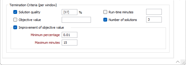
Solution quality
(Optional.) Select to terminate the solver when a specified solution quality is achieved.
As an integral part of its operation, the solver determines and maintains an upper limit for the total profit that could be produced from any solution that satisfies the design parameters. Expressing the total profit produced from the solver’s current solution as a percentage of this upper limit provides a measure of the “quality” of the current solution.
(Optional.) Specify the minimum quality (0.00% <= x <= 100.00%) of a feasible solution to be achieved before the solver is terminated. If not specified, the solution quality defaults to 95%.
Objective value
(Optional.) Select to terminate the solver when a specified value of the objective (total profit from the mined stopes) is achieved.
Specify the minimum total profit to be produced from a feasible solution before the solver is terminated.
Improvement of objective value
(Optional.) Select to terminate the solver once it becomes clear that significant additional time may be required to produce solutions with higher total profits.
Minimum percentage
(Improvement of objective value only.) Specify the minimum percentage improvement in the total profit between successive solutions.
Maximum minutes
(Improvement of objective value only.) Specify the maximum number of minutes of processing time that may be used to produce the minimum improvement in the total profit.
Example: The default settings of Minimum percentage = 0.01 and Maximum minutes = 15 specify that, if the improvement in the total profit between the current solution and the previous one is less than 0.01% and more than 15 minutes of processing time was required to achieve that improvement, the solver should be terminated and the current feasible solution should be used.
Run-time minutes
(Optional.) Select to terminate the solver after a specified number of minutes has elapsed.
Specify the maximum number of minutes of processing time to be used before the solver is terminated.
Number of solutions
(Optional.) Select to terminate the solver after a specified number of solutions has been found.
Specify the maximum number of solutions to be found before the solver is terminated.
Log file
Double click in the field of use the Select button to optionally select or create a log file for the solver.
Terminating the Solver Manually
Ensure that the instance of the application for which you would like to terminate the solver has the active Windows focus.
Press ESC to terminate the solver manually at any time. You will be prompted to confirm the interruption of processing. Click “Yes” to direct the solver to terminate at the first available opportunity.
Depending on the size of the block model, the number of blocks in a minimum stope, and the setting of Project | Options | System | System Options | Resources > Multi-core Processing > Limit the number of cores the application can use, terminating the solver may take some time. You may need to be patient during this process if you require access to the solution.
Tip: You can use the Windows Task Manager to monitor the performance of the computer as the solver is terminating and to gauge how much additional time may be required to complete the process. CPU % Utilization and Memory will both decrease as the solver terminates each of its search threads.
After the solver has been terminated, if a feasible solution with a quality of at least 30% is available, you will be prompted as follows:

Click “Yes” to process and load the current solution from the solver.