Example

In this topic, let's look at a simple example which illustrates how data flows are setup and run.

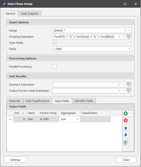
Suppose we want to write different Size values to the leaf nodes in the Deposit table. To be able to write any results to the Deposit table, folders and fields referenced by the data flow need to be selected so that values can be written to the records in the table:

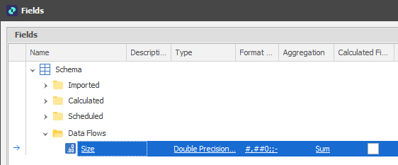
The Aggregation property of the Size field is set to Sum so that size values can be viewed at a higher level than the leaf nodes of the table.

In this example, table parameters are used to query the data table. if records are in a default range, then the value 1 will be written to a Size attribute (see Parameters below). If records fall within a specific sub-range, then the value 2 will be written to the Size attribute.

Table Parameters

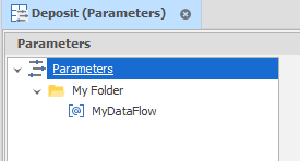
To achieve this, a parameter is added to the Table Parameters of the Deposit table (available on the Home tab, in the Data group or via the table's right-click option).

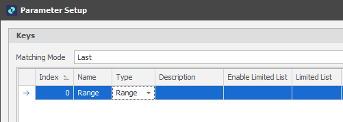
Keys

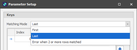
When you right-click on the table parameter and select Settings, a Matching Mode setting determines which parameter row is applied when multiple criteria are matched:

Mode	Description
First	When retrieving table parameters, if multiple criteria are matched, select the FIRST matched entry (top of the list).
Last	When retrieving table parameters, if multiple criteria are matched, select the LAST matched entry (bottom of the list).
Error	If multiple criteria are matched, return no result or raise an error, depending on the context.

A Range Key is added. This is just a way of making sure that we are looking up a unit based on whether or not it belongs to a range:

Note: To make the cells in the Table Parameters window editable, you may need to select Unlock on the Home tab, in the Parameters group . To avoid inadvertent changes to the cells in the Parameters window, Locked () is the default.

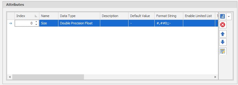
Attributes

The second part of the Parameters Setup window is where Attributes are defined. Attributes are matched to the fields in the underlying data table and are used to generate the unit results when the data flow is run.

Note that data flows do not operate directly on the leaf nodes of the underlying data table, which belong to a rigid tree hierarchy. Instead, units are derived from the leaf nodes of the table and are able to be manipulated (merged or split) using expressions.

In this example, a "Size" attribute (with a Double data type) is created to match the Size field that was added to the underlying data table:

To assign Size values depending on whether records fall within the default range (all levels) or a specified sub-range, two parameter rows are added:

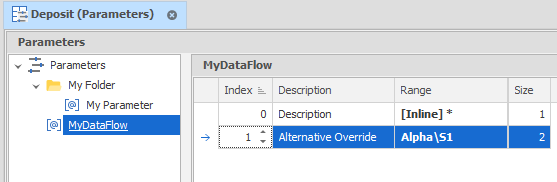
In the first parameter row, all levels are selected and a Size value of 1 is specified. In the second parameter row, a sub-range (Alpha\Strip 1) and a Size value of 2 are specified.

Since the Matching Mode is set to LAST, a Size value of 2 is assigned to all records that fall within the sub-range. A Size value of 1 is assigned to all records outside of the sub-range (since only the first range criterion is met).

Once table parameters have been setup, they can be referenced in the data flow.

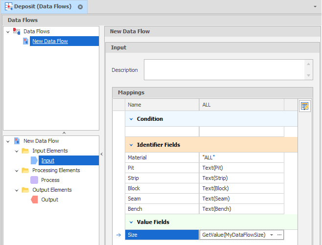
In this simple example, a data flow has been set up with just one ("Size") Value Field. In more complex data flows, multiple (Text) Identifier Fields and (Numeric) Value Fields will typically be specified.

Once the data flow has been setup, Input, Process and Output elements can be added to the data flow diagram (as described in the Data Flows topic). In this simple example, there is just one element of each type. More complex data flows will typically have multiple inputs, processes and outputs.

Input

For the Input element, the Value Field specified in the Settings is mapped to the Size values that will be passed from the parameters that were setup for use by the data flow.

Processing

For the Processing element, a new code snippet is added.

In the example below, a FOR loop is used to iterate over the units. For each unit, its record needs to be retrieved from the underlying table. A good practice is to make sure that every unit has an Input Node.

If the input node is NULL (there are examples where units are created from scratch) then that unit is skipped. Otherwise, for the units that are processed, the code snippet continues to look up the parameters that will be used to write the unit Size.

The code snippet can be tested by hitting the Recalculate button at the top the Preview pane. Tip: At this point, it may be necessary to use the Column Chooser (right-click on a column header) to locate the "Size" field.

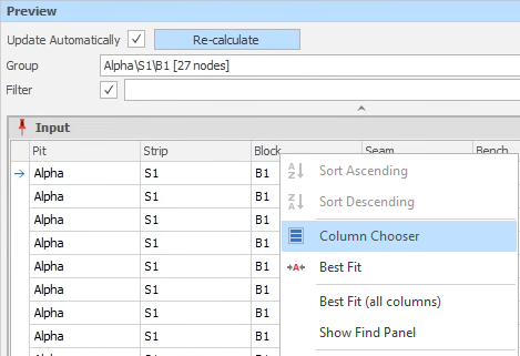
The Preview pane shows "the Before and After" of any processing. When Alpha\Strip 1 or a sub-range of Alpha\Strip 1 is selected as the Group, we can see that the number 2 has been written to the Size attribute since this is within the range that was defined as having an "alternative" size:

The preview for all other units (outside the range Alpha\Strip1) are assigned a Size value of 1.

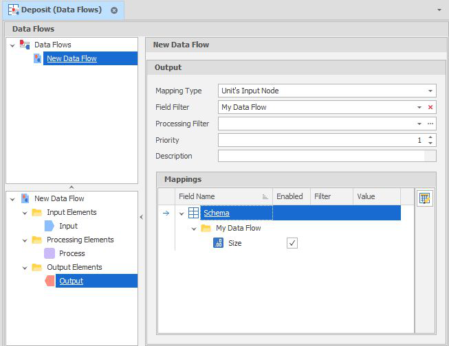
Output

Units, on their own, do not affect the model unless those unit values are written back to the underlying table. This is where the Output element comes in

In this example, the Mapping Type is set to "Units Input Mode" . In other words, wherever a unit is derived from is where the unit value is written back to.

The Field Filter is also set so that we only see the fields associated with the data flow:

Run

Once the data flow setup and a preview of the results is complete, the data flow can be run by selecting an option on the Home tab, in the Graph group:

	Run	Run the current data flow
	Run With Filter	Run the current data flow with a specified range.
	Run All Data Flows	Run all data flows in the order they are listed.

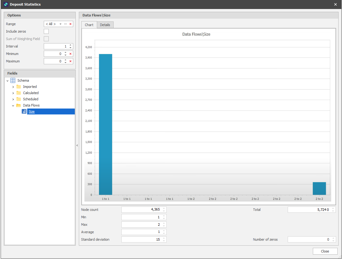
To check that values that have been written to the Size field in the data table, right-click on the table and selecting Utilities | Field Statistics: