Chi-square

Chi-square is a statistical test that measures the “goodness of fit” of the data. That is, it determines if the set of data under investigation (the sample) matches the chosen distribution. Depending on which function you use, the sample may be compared to a Uniform, Normal, Log-normal, or Exponential distribution by setting the Scale or Distribution option as required.

The Chi-square test divides the data set into bins with a fixed width. Bins including fewer than five samples are combined with the adjoining bins to produce a robust calculation, which most often happens at the tails of the sample data distribution.

For each bin, the expected number of observations is calculated and then subtracted from the measured number of observations in that bin. The result is squared and then divided by the expected number of observations. Lastly, the results for the bins are summed to produce the Chi-square test statistic. This number can then be tested against the critical value to determine if the sample data matches or does not match the test distribution. Critical values for different combinations of degrees of freedom and significance level can be obtained from standard Chi-square statistical tables.

If the calculated value of Chi-square test statistic is less than the critical value, then you can accept that the sample matches the distribution it was tested against. Alternatively, you can draw the same conclusion if the p-value is greater than the significance level.

Otherwise, if the calculated Chi-square test statistic exceeds the critical value, or if the p-value is less than the significance level, then you can reject the distribution.

The significance level is a measure of how unlikely a value you will tolerate before rejecting the distribution. Although the significance level can range anywhere from 0 to 100%, typical values are 1%, 5%, or10%, with larger values representing a more rigorous test.

The p-value is the probability associated with the critical value for a given degree of freedom. It is a test against the sample data matching the distribution; as the p-value becomes smaller, the sample data becomes less likely to match the distribution.

Degrees of freedom (DF) is equal to the number of bins minus 1. It is adjusted accordingly whenever bins are combined, which may result in a smaller than expected DF value.

When testing geological data against a normal distribution, you may find that you are frequently rejecting the distribution. However, if the sample distribution has a single peak and is roughly symmetrical, then the assumption of normality generally produces acceptable results (Wellmer, 1998, p.40). This concept may also be extended to the results of a decomposition: if the Chi-square value is relatively low, and the fit between the data and model looks right, with matching peaks and valleys, you can treat the decomposition as suitable.

The Chi square value is defined as:

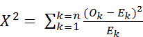
Where is the number of observations in bin K

and is the expected number of observations in bin K

Reference: Wellmer, F-W., 1998. Statistical Evaluations in Exploration for Mineral Deposits. Springer-Verlag, Berlin. 379pp