Lerchs Grossman Lowest Label
The Lerchs-Grossman algorithm is an industry-standard optimisation technique used in mining and exploration to detect the true optimum pit.
For a deposit which is represented as a block model, in terms of ore grade or block revenue, the slopes of the pit are specified in terms of the overlying blocks that must be removed to provide access to each block within the block model.
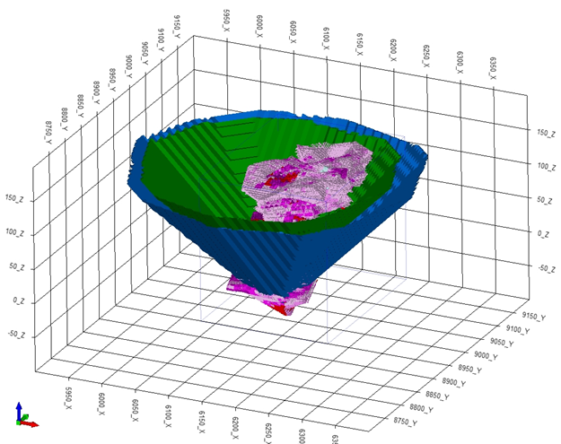
In the Lerchs-Grossmann algorithm, directed arcs indicate which blocks need to be removed before a particular block can either be mined and processed, or, be dumped as waste. The Lerch-Grossmann algorithm and a Lowest Label Pseudo-flow (LG/LL) approach is used to undertake an optimisation.
This implementation is mostly based on the paper:
Hochbaum, D S, 2001, A new-old algorithm for minimum cut and maximum-flow in closure graphs, Networks, special 30th anniversary paper, 37(4):171-193.
The value of a waste block is usually defined by the cost of mining and disposal (dumping, reclaiming, etc). A negative value indicates a loss. The value of an ore block is usually defined by the net revenue from the mineral sale, minus the costs associated with mining and processing all the material in the block.
An ore block will have a negative value if the costs are greater than the net revenue. It makes sense to consider a block as an ore block if the loss is less than it would be if it were treated as a waste block. In general, the pit optimisation process treats negative blocks as waste, and positive blocks as ore.
The ultimate pit is a pit which gives the highest possible undiscounted surplus between net revenue and total operating costs, but which does not consider either scheduling constraints or discounting.
The optimal pit gives the highest possible net present value, taking into account all operational scheduling constraints (annual mining and processing productivity), discounting and recurring capital costs. The ultimate pit can be considered as the optimal pit, but only for a deposit with a short mining life (approximately 3 years). If the life of mine is longer, it is necessary to generate nested pit shells and do an analysis of optimal pit shells.
In order to determine the discounted optimal pit, a subsequent analysis of nested pit shells is necessary. Nested pit shells are the ultimate pits that are generated using identical input data, except for the price of material produced, to which multipliers (Revenue Adjustment Factors - RAF) relative to the base price of material produced are applied.
Optimal pit analysis
Optimal pit shell analysis is the analysis of the ore reserves, waste tonnage, metal production and cash flow for each of the nested pit shells. The ore reserves in each nested pit shell are calculated using a fixed metal price.
The analysis of nested pit shells allows the optimal pit shell to be selected, and the future discounted financial cash-flow to be determined, taking into account the discount rate and other parameters such as recurring expenses.
Three methods can be used to determine the mining sequence for the pit shells:
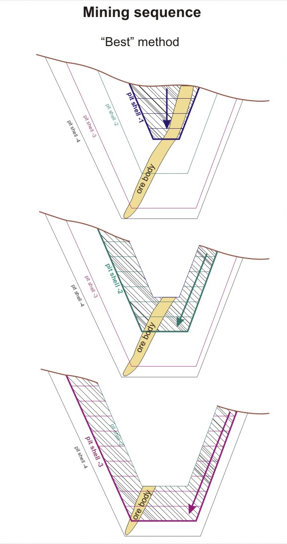
Best case
The “best” method assumes that the pit shells will be mined consecutively (initially the first one, then the second one, etc.). ![]() Show me...
Show me...
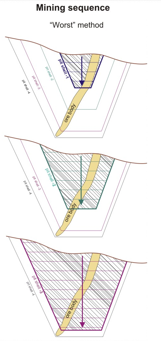
Worst case
The “worst” method assumes that each pit shell will be mined completely from top to bottom, without taking any other pit shells into consideration. ![]() Show me...
Show me...
In real life, neither the "best" or the "worst" method is used on its own and the true optimal discounted pit is selected as the average between:
- the pit with the maximum NPV using the “best” method
- the pit with the maximum NPV using the “worst” method
Alternatively,
- the pit with the maximum NPV can be identified using a "Constant lag" (real life) method:
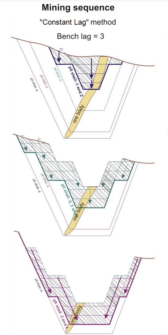
Constant lag
It is often difficult to select a pit shell with the highest achievable NPV (the optimal pit shell), when the difference between the NPV curves for the "Best" and "Worst" methods is significant. It is now possible to use a specific method to model a more realistic mining sequence and its cash flows.
"Constant lag" assumes that the pushbacks will be mined in consecutive order, as per the "Best" case scenario, but also considers the number of benches that need to be mined on each pit shell.
If the lag is set to 0 (zero), each push-back is completed before the next is started, so the analysis works exactly like the "worst" case. Obviously, increasing the bench lag takes the mining sequence closer to the "best" case.
If the lag is 3, then bench (n-3) of the second pit shell will be mined at the same time as bench (n) of the first pit shell. In other words, the second pit shell is not mined until the third benches of the first pit shell are mined out, and the third pit shell will only be mined when the third benches of the second pit shell have been mined out completely.
The Pit Optimisation process will now report the MIN-MAX ranges of the benches (which are the Upper and Lower benches in each pushback). Because the "Constant lag" method can be used for preliminary scheduling, it is necessary to flag the block model cells by the period they will be mined and the pre-pushback to which each block belongs.
An illustration of the "Constant lag" method is ![]() shown in the following diagram...
shown in the following diagram...
Results
The following values are calculated as a result of the pit optimisation process:
- Pit – the number (and name) of each nested optimal pit shell (i.e from 1 to 30).
- Period – the pit shell mining life, i.e. from 0 to 6 (7) for the best case of mining sequence. A value of 5, for example, indicates that the pit will be mined for 6 years.
- Waste – both rock waste and uneconomic ore (internal dilution).
- Ore – ore weight in the pit shell without dilution and mining losses. Both ‘total’ and ‘value according to processing method’ are shown.
- Grade – average metal grade after mining, with mining dilution. Both ‘total’ and ‘value according to processing method’ are shown.
- Metal recovery – metal as a product, i.e. after mining and processing. Both ‘total’ and ‘value according to processing method’ are shown.
- Revenue – income from the sale of the recovered metal. Revenue is shown for the two mining sequence methods.
- Cost – the summary of costs (expenses) of mining operations and ore processing operations, shown for the two mining sequence methods.
- Profit value – the difference between the revenue and mining and processing costs. It is shown for the two mining sequence methods.
- NPV – the discounted difference between the revenue and the mining and processing costs, including capital and replacement capital costs (if used). In other words, NPV is equivalent to the sum of all discounted cash flows. The NPV is shown for the two mining sequence methods.