Mining Planner
Micromine has two types of scheduling project:
Operational
One of the requirements of the mining model is to generate a mine plan which represents the tonnes and grade (quality) in both a graphic and a tabular form. Scheduling involves defining the mine layout as a series of mining blocks, sequencing the order in which those blocks will be mined, and mapping this to a timeframe in order to meet periodic targets.
The Scheduler has provision for sequencing and the allocation of resources to the mining blocks. With a time component added, the mining blocks can be visualised (and animated) in the Vizex window. Associated attributes (tonnes, grades, equipment etc.) may be interrogated or used for colour coding. The information can also be represented in a Gantt Chart window, or as a report. The Vizex and Gantt Chart windows are linked, and fully interactive.
Once tasks have been defined for the schedule, you can use the Gantt Chart to assign resources to those tasks, set start times for tasks, remove tasks, define the dependencies and any lag, between tasks and specify task groups. If you have used applications such as Microsoft Project, many of the features of the Micromine Gantt Chart will be familiar to you
Strategic
(These notes describe an open pit mine. The same principles apply to an underground operation.)
By considering all the mining blocks of a proposed pit design, the strategic scheduler uses an optimisation process to determine which mining blocks should be mined in which period. The planning horizon for the optimisation is typically ten years (or more). The operational scheduler is then used to determine how best to mine the contained material for the upcoming period. Although the period can be user-defined, it is normal for it to be a year.
The optimisation can be re-run at any time, excluding any material that has already been mined. This becomes an iterative process over the life of mine.
The optimisation process is driven by an objective and is subject to various constraints. Usually the objective is to maximise discounted metal production. There are two types of constraint:
- Dependency constraints (accessibility):
- Horizontal: the order that blocks on the same bench will be mined.
- Vertical: a block cannot be mined unless the blocks above it have been mined.
- Stage: if the mine plan is staged, then blocks from a previous stage must be mined before blocks from the next stage can be mined, based on a bench lag.
- Capacity constraints (per period). Examples are:
- Mining capacity - maximum amount of rock which can be mined in one period.
- Processing capacity - maximum amount of ore that can be handled by the processing plant in one period.
- Average grade (weighted average) with minimum and maximum
- Grade constraints:
- The minimum and maximum (weighted average) grade per period.
As well as the objective and constraints, a period and time horizon need to be defined. Typically the period is a year and the time horizon is the expected life of mine.
The production schedule is optimised by using a mathematically proven Mixed Integer Programming (MIP) solver. Running the optimisation process will define which blocks should be mined in which period, to achieve the objective.
On completion, the Mining Period attribute for each task is populated and a Start date and Finish date are calculated.
These dates indicate a possible mining sequence, based on the period and the horizontal, vertical and stage dependencies. By doing this, the tasks can be animated to give a realistic indication of what the mine will look like at any future date.
The Solver
Micromine includes a built-in solver which is highly optimised with support for multiple processor cores. The number of cores that can be utilised is dependent on the Limit the number of cores Micromine can use setting on the Resources > Multi-core Processing tab of the Options | System form.
A less optimised solver is provided for backward compatibility (select the Use legacy solver check box).
Sliding window
The built-in solver has the option of defining a sliding window. This breaks the problem into smaller, overlapping time horizons in order to reduce the solution time.
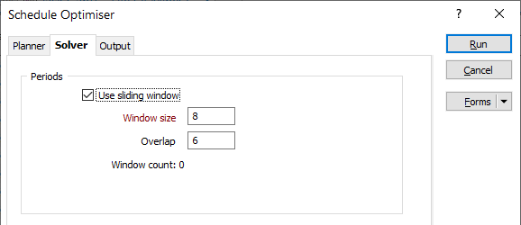
For example:
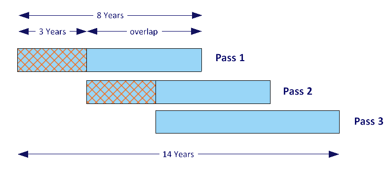
If the time horizon is 14 years, then choosing to use an 8 year sliding window with a 5 year overlap, will reduce the problem into 3 smaller parts. The first “pass” will consider all mining blocks, using a time horizon of 8 years. This solution will determine the blocks mined in the first 3 years (Window size - Overlap).
The second “pass” will exclude these blocks from the problem and this solution will determine the blocks to be mined in years 4 to 6.
The final pass will solve for years 7 to 14.
In practice, the solution obtained using sensible sliding window values will not be significantly different to the solution for all mining blocks across the complete time horizon. However, the performance gains can be significant. Considering the example above, common sense suggests that knowing which blocks will be mined in years 9 to 14 will have little effect on the blocks mined in years 1 to 3.
Preparation
The long term scheduler requires mining blocks that are “indexed”, based on a predefined 3D grid of rows, columns and benches. To do this there is a new function Create Mining Blocks. The input is a pit solid. Parameters define the grid size, orientation and the bench levels. Running the function generates indexed mining block solids (wireframes).
To assign material grade bins to each block, the Grade Tonnage Report has been enhanced to enable multiple grade categories to be written to a wireframe. The feature used to do this is called a material set.
Workflow Summary
- Start with a pit solid and a block model.
- Convert the pit solid into mining blocks using the Create Mining Blocks function on the Mining tab, in the Task Preparation group.
- Run the Grade Tonnage Report on the Wireframe tab, in the Report group,to attribute the grade values from the block model to each mining block.
- Import the mining blocks and their attributes into a Strategic schedule.
- Define dependencies for the tasks.
- Define the capacity constraints and the objective.
- Run the solver.
- Display the result as an animation and use this as a reference for Operational (short term) planning.